Full description of the game "Small Evolution".
Small Evolution - Introduction

The key question scientist tried to answer by using evolutionary game theory was: why is it that the ratio between predators and prey is approximately equal in a population? Studying some mathematical models, they came to the conclusion that the fitness (ability to achieve the life purpose) of a species depends on the distribution of predators and prey in the population.
When there is a greater number of predators in the population, paradoxically prey have a higher individual fitness - predators have less opportunity to find them and also competition between predators is growing. In reverse, when there are more prey in the population, predators have a higher individual fitness - there is an abundance of food and less rivals. Scientists point out that, due to this, across the subsequent generations the ratio between predators and prey hovers around a certain value.
The most important conclusion that comes from the analysis of evolutionary games is that: individual fitness depends upon the relative number of predators and prey in the population.
Small Evolution - The Rules

A classic evolutionary game for The Physics of Life - a model of a society consisting of independent objects absorbing the available resources.
The game is imposed on a population composed of a number of players (n). For a period of time all the players are randomly matched in pairs and play against each other in a contest called a single-meeting game. Depending on the strategies used, each player gains or loses points. After each single-meeting game, each player adjusts his account, wins and losses, and prepares for the next meeting after the pairs are redrawn. The most important factors of this game are the rules of selection and duplication. Occasionally, sometimes after three single-meeting games, sometimes after a million (nobody knows when), the selection and duplication occurs. When it happens all the players are ranked according to points gained. Then the top 50% of players are selected for the subsequent games. The bottom half is rejected and no longer take part in the game - you can say that they are annihilated. Those who pass the selection are duplicated and gameplay restarts from the beginning. As you might notice, after this operation, the population remains at the same level of output. These cycles repeat ad infinitum.
To be exact, let's name:
-
Population level
 - the studied population consists of Thieves and Producers. The premise of the game is that the population level remains constant. The number of participants equals N.
-
Composition of the Population
 - the studied population consists of Thieves and Producers. These titles define the character of the individual population members. Therefore, the Thieves are only able to steal the points whereas the Producers create them.
-
Single meeting game
 - when two participans meets within the game, a single meeting game occurs. The result of this game is that both parties gain or lose points. The Payoff Matrix shows how the points are designated according to the character of the participants. In a classic Payoff Matrix, proposed by John Maynard Smith, when Thief meets Thief, both of them lose 25 points.
-
Points
 - in evolutionary games these points are called: "survival points" or "sharable resources". Immediately, some simple questions occur:
- From where do these points come?
- Why as a result of a single meeting game, both participants can take from an external reserve of points to and share them among themselves?
Imagine that a Small Evolution game is being played between foxes and hares in a grass clearing. The grass is a life resource [resergy] for the hares and for foxes, the hares are. In turn, for the grass the life resources are: animal droppings and solar energy. The Sun is, in fact, the ultimate and primary repository of points of survival.
A meeting of two foxes results in the irretrievable loss of points - neither of them gain nothing yet lose their time. When a fox meets a hare, and is able to catch it, it will profit from all the resources of the hare. When two hares meet they can reproduce, increasing their number which, therefore, increases the resources available for the foxes.
Generally speaking the points in evolutionary games are resergy - resources required for survival and reproduction, resource needed to achieve life purpose.
-
Round
 - it is a random pairing of all participants and the performing of single meeting games. The gains and losses are added to each participants individual account.
-
Selection
 - the selection process selects a certain percentage of individuals, eg. 50%, who have achieved the highest number of points. The rest are eliminated. After this, the population undergoes the process of the Restoration of the Population.
-
Cloning
 - it is the process of creating exact copies of an individual participant. For example, cloning a Thief results in two Thieves.
-
Restoration of the Population
 - it is the process of cloning selected individuals in order to maintain the population level.
As you will note, the simplest example is when 50% of the individuals are selected, then each of them is cloned - so one creates an identical copy of himself and thus the population is restored after the selection process.
In contrast, when the strength of the selection function differs from 50%, the process of restoring the population becomes complicated and requires a precise definition. For example, when the selection function is strong (eg. selects from the top 10%) the individuals are cloned repeatedly, but when the selection function is weak (eg. selects from the top 90%), then most of those who managed to pass the selection will not be cloned. Beacuse only 10% of the population needs to be replaced;
-
Cycle
 - sequence of rounds culminating in selection and Restoration of the Population.
-
Cycle length
 - the number of rounds taking place in a single cycle, which is not constant
-
Selection function strength
 - the percentage of individuals from the population selected for the process to restore the population.
-
Payoff Function
 - a function whose arguments are the strategies used by individuals (players) involved in the single meeting game, and the resulting number of points awarded to each of them. In the classic example, proposed by John Maynard Smith, this function is represented by a payoff matrix.
-
Payoff Matrix
 - this is a special case of payoff function. Payoff matrix determines how many points are awarded to the individual depending on which strategy has been applied by him and his opponent in a single meeting game. Specific examples of such matrices are: the "Classic Maynard Smith" payoff matrix and the "Realistic" payoff matrix .
Small Evolution - Classic Maynard Smith's payoff matrix

Basic assumptions:
A good example of the classic game theory proposed by John Maynard Smith, uses two types of players (producers and thieves), and a payoff matrix as shown below:
|
|
||
|
|
|
|
| Thief | Thief loses 25 (-25) Thief loses 25 (-25) |
Thief gains 50 (+50) Producer gains nothing (0) |
| Producer | Producer gains nothing (0) Thief gains 50 (+50) |
Producer gains 15 (+15) Producer gains 15 (+15) |
The goal of the analysis of the "Small Evolution" of such a payoff matrix, is to answer the question: "Which of the strategies is better - the producer or the thief?". Or, which will give a higher chance to pass through the selection and consequently be cloned. Note that the adjective "better" is only due to the rules of this game - better are those, who in the conditions imposed by this game, accumulate more points. When the rules of the game change, those who succeeded before may not succeed in the new condition.
Analysis starts from the occurence when the population is made up of many producers and only one thief. The thief collects points in every single meeting game, and ranks at the top of the list after the first meeting, and remains there unbeaten until selection. Being at the top will guarantee his selection and cloning himself and the strategy he uses. From now on we have two thieves (the original and the clone) in the population whilst the rest are Producers.
Now consider a population consisting of one Producer and many Thieves. The producer does not lose points when meeting a Thief. However, when two Thieves meet they lose points. This means that the Producer will be high enough to pass the selection, and be cloned. In the second round there will be two of them in the population. So the tendency for the number of producers to increase is observed.
Classic mathematical analysis:
One Thief in the population of Producers duplicates, as does a single Producer in a population of Thieves. It means that, for a Classic Maynard Smith Payoff Matrix, at some point the ratio of Producers and Thieves will reach an equilibrium. It is calculated as follows:
  Suppose x is the ratio of the number of Thieves to the number of all participants,
  the sum of the number of Thieves and the number of Producers.

  E(Z) – The value of the points earned by a Thief during a meeting with
         a random participant from the population
  E(P) – The value of the points earned by a Producer during a meeting with
         a random participant from the population
  P(Z) – Probability of encountering a Thief during a meeting with
         a random participant from the population
  P(P) – Probability of encountering a Producer during a meeting with
         a random participant from the population

  P(Z) = x
  P(P) = 1 - P(Z) = 1-x
  E(Z) = P(Z) * (-25) + P(P) * 50 = -25*x + 50*(1-x) = 50-75x

  E(P) = P(Z) * 0 + P(P) * 15 = 15*(1-x) = 15-15*x
  E(Z) = E(P) which means that the average number of points earned by a Producer
         or a Thief will be equal: 50-75*x=15-15*x

  Hence x=7/12
Using a Classic Maynard Smith Payoff Matrix in the subsequent rounds, the number of Thieves will stabilize at 7/12 of the population and the number of Producers at 5/12. The tendency of this system is to maintain a steady ratio of Thieves to Producers at around 7:5. What is the conclusion of this analysis? In life, as in our game, there is no absolutely right way to go, or one winning strategy that guarantees success in all conditions. Any strategy not only depends upon itself, but also on the environment around it. Sometimes the Thief's strategy is better, sometimes it is the Producer's and sometimes they are both equal. This is a very important conclusion, especially for those who think that fully understanding life is inextricably linked with discovering one single strategy that will allow you to win permanently! Changing external conditions may make a strategy that works well today turn out to be useless tomorrow.
Reductionist thinkers look at this analysis and fully agree that the number of Producers to Thieves always stabilizes at this level.
However, very interesting results are shown by computer simulations. It reveals that it is not so simple. That's why I strongly recommend to study Small Evolution - Simulations.
Small Evolution - Simulation programme

The programme "Small Evolution" is a computer simulation of the abovementioned game Small Evolution.
This chapter includes:
-
- Description of basic settings
- Description of simulation windows
-
Technical description of the programme:
- Description of the simulation
- Description of calculating the average
- Description of the recovery of the population algorithm
Instruction manual:
Basic settings
After running the programme, the Initial Settings Screen appears:

Initial Settings Screen of the "Small Evolution" simulation programme.
Prior to starting the simulation you should set the initial values. They are grouped as follows:
-
Payoff Matrix - the programme starts with the values from the previous session. When you click on the [Default values], John Maynard Smith's original values will be applied. The section of payoff matrix {Payoff Matrix} is enriched with two additional columns showing the values of mutants. In the above screen, you can see a column with the values of the Mutated Thief MT, while the column MP (Mutated Producer) remains invisible.
-
Population Level and Composition of the population - these parameters are introduced in the section {Population}. You adjust the initial number of Thieves and Producers by moving the sliders. The population size is calculated automatically and shown in the window {Population}.
-
Mutation Level. The programme allows you to enter one individual mutant. A mutant differs from its predecessor, as are the points given for an action. The points can be affected either when meeting another Thief, meeting a Producer, or both. The programme allows you to make a mutation of both dimensions, improving or deteriorating the points given. Entering new values can be made by percentage or by entering the values you want.
The Mutant is introduced by clicking the appropriate radio button in the {Mutation} section, and values of the mutation are adjusted in additional column of the {Payoff Matrix} which comes up automatically. -
Selection strength - this parameter is set up in the section {Selection strength}. If you set it to, say, 80%, this means that to the restoration of the population phase will only devote the 20% of individuals who have accumulated the most points in each cycle
-
Cycle Length - this parameter is set up in the section {Length of cycle}. For each cycle the number of rounds is determined randomly by the programme. In the section {Length of cycle} you can specify the range. In the example above the number of rounds will be not less than 1 and not more than 1000.
-
After setting up all the starting parameters you are ready to start the simulation by clicking the {Simulation} button.
Simulation window
Used to show the population changes over time simulated by the game "Small Evolution".
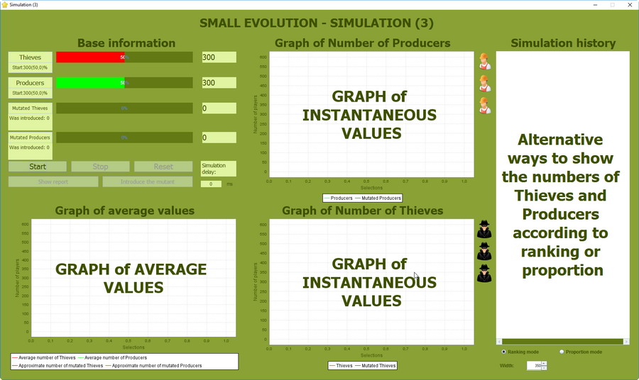
Simulation window of the game "Small Evolution" before starting the simulation.
Elements of the simulation window:
-
Basic information - this area displays the number of Thieves and Producers and the number of Mutants, if and when they are introduced to the game.
-
Simulation controls:
- {Start} - starts simulation;
- {Stop/Restart} - which allows you to pause and resume or stop the simulation. Only when you pause, you can introduce the pre-defined Mutant;
- {Reset} - which allows you to start the simulation again from the beginning;
- {Show Report} - it shows the report of the simulation;
- {Introduce the mutant} - by clicking this button, only when the simulation is paused, we can introduce the pre-defined Mutant;
- {Simulation delay} - the basic setting mean that the simulation runs very quickly. This allows you to slow the simulation down;
-
Graph of average values - it shows the average values of the number of Thieves and Producers in the simulation. The peaks and the troughs indicate the end of a cycle.
-
Graph of number of Producers - shows the changes in the number of Producers after each cycle.
-
Graph of number of Thieves - shows the changes in the number of Thieves after each cycle.
-
Simulation history window - the window graphically shows the history of all rounds and all cycles. This information is shown in one of two ways:
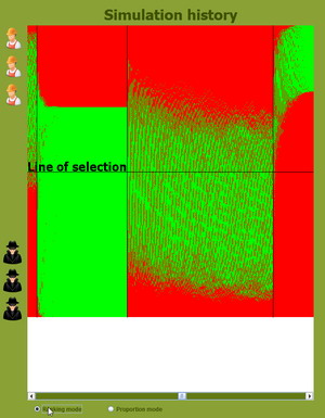
- In the {Ranking mode} the red pixel represents a Thief, the green one, a Producer. The pixels represent the ranking, from top to bottom, according to the points gained by each participant. If, at the top of the list, there are 2 Thieves followed by 6 Producers, then the graph will show 2 red pixels at the top and 6 green ones directly underneath.
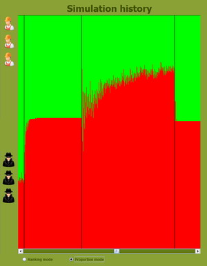
- In the {Proportion mode} the display shows the proportion of Thieves to Producers. But be aware: This does not represent the proportion of the whole population, but only those who have the potential to selected for the next round.
In the simulation screen you are able to adjust the width of the Simulation history window. To do this, introduce a new setting of pixels into the field labelled "Width" in the bottom-right corner.
Technical description of the programme:
The simulation
Algorithm of the simulation:
- Based on the data entered by the user, a population is created, a list of Thieves and Producers is created.
- Only Thieves and Producers are available.
- The Cycle Length is determined in a random manner using Random.nextInt function. The boundaries for this value are specified by the user in the "Initial Settings" window.
- The round is completed.
- The rounds counter is increased by one.
-
The ranking of individuals is determined on their accumulated points. This ranking is shown in the "Simulation History" window, where each bar has a width of one pixel. There are two visualizations possible in this window:
- as individuals are ranked (each pixel represents one individual, vertically)
- in the form of proportion of those who have the potential to be selected for the next round
-
If the rounds counter is equal to the Cycle Length then:
- The rounds counter is reset
- Selection is performed
- The population is restored using the restoration algorithm.
- In the restored population all individuals accounts are reset.
- The programme calculates the statistical values and updates charts.
- The programme starts the next Cycle. The programme goes to point B.
- If the rounds counter is less than the Cycle Length the Cycle is continued. The programme moves to point C.
Calculating the average 
- The programme calculates the numbers of each individual strategy (Thieves / Producers / Mutated Thieves / Mutated Producers) for each Cycle and memorises it.
- The arithmetic means of these values are shown in the "Graph of average values". If we use Thieves to explain further, we add the values of each Thief after each cycle, and then divide this total by the number of cycles.
Restoration algorithm
- The selected Participants are ordered randomly. This is named as the list of predecessors of the new population (PNP).
-
Every Participant from this list is analyzed individually in order:
- The Participant is cloned and only the Clone is added to the New Population.
- If the number of individuals in the New Population is equal to the population level, the process is stopped. The programme moves to point C.
- If the number of individuals in the New Population is less than the population level, the next Participant from the PNP List is analysed. If all Participants from the PNP List have been analysed before the Population is fully restored, the programme reverts back to the top of the PNP List
- The List of the Restored Population is returned.
Introducing a Mutant
- The Mutant is introduced after the restoration algorithm. The consequence of this is that each Participant, including our new Mutant, starts at the same value level, zero.
Programme downloading 
 A computer programme "Small Evolution simulation program" is available Pro Publico Bono on a Creative Commons License. This means that users provide the following rights:
-
Attribution. (BY) Licensees may copy, distribute, display and perform the work and make derivative works and remixes based on it only if they give the author or licensor the credits (attribution) in the manner specified by these.
-
Non-commercial. (NC) Licensees may copy, distribute, display, and perform the work and make derivative works and remixes based on it only for non-commercial purposes.
-
Share-alike. (SA) Licensees may distribute derivative works only under a license identical ("not more restrictive") to the license that governs the original work.

Small Evolution - Simulations

This chapter shows some simulations and discusses how the change of a selected parameter changes the composition of population in subsequent cycles. We will study the influence of variations of:
cycle length,
population level,
selection strength,
and the changes in the composition of the population after the introduction of:
a Negative Mutant,
a Half-Positive Mutant,
a Full-Positive Mutant.
The remarks and conclusions will be given at the end of this section.
Simulation without mutation - varying the Cycle Length:

The amended parameter is the cycle length, which is the number of rounds before selection and the restoration of the population. Let's see how it affects the composition of the population.
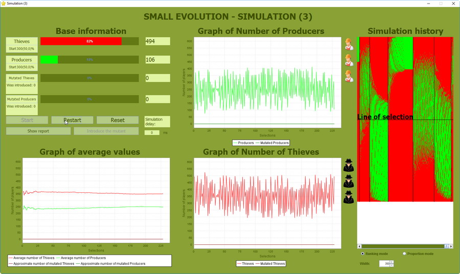
Analysis without mutation - cycle variance from 1 to 100 rounds
When the cycle length varies between 1 and 100 rounds, a relative stability of the population is observed. The analyzed population consists of 600 individuals. The number of Producers can be between 100-400, and 200-500 Thieves. You can see that the simulation confirms the correctness of the theoretical model.
Analysis without mutation - cycle variance from 1 to 400 rounds
When the cycle length varies between 1 and 400 rounds, a relative stability of the population is observed. The analyzed population consists of 600 individuals. The number of Producers can be between 1-450, and 150-599 Thieves. You can see that the simulation confirms the correctness of the theoretical model. It is curious that both populations are touching their limits by increasing the number of rounds. The Producers are threatened by extinction, and the Thieves are close to dominating the population.
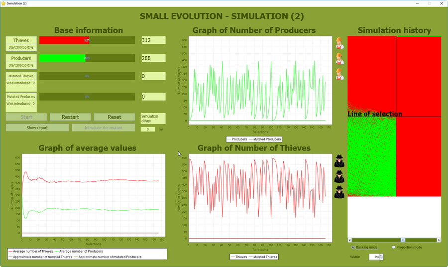
Analysis without mutation - cycle variance from 1 to 600 rounds
When the cycle length varies between 1 and 600 rounds, a relative stability of the population is observed until the latter stages. The analyzed population consists of 600 individuals. The number of Producers can be between 0-450, and 150-600 Thieves. In one moment, however, the simulation diverges from the theoretical model. The reason of this is that the theoretical model does not take into account the amplitude increase resulting from the number of rounds. Note that the Producers become extinct around the 325th cycle.
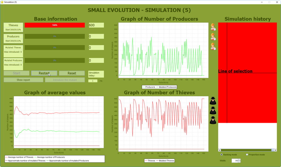
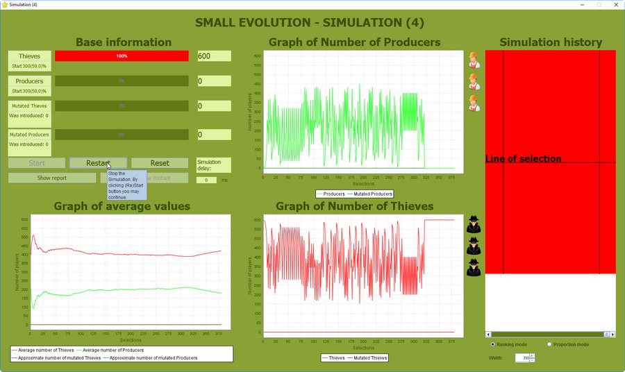
Analysis without mutation - cycle variance from 1 to 800 rounds
When the cycle length varies between 1 and 800 rounds the simulation diverges from the theoretical model quicker than before.
Note that the Producers become extinct around the 145th cycle.
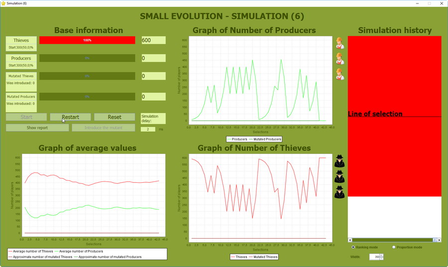
Analysis without mutation - cycle variance from 1 to 1000 rounds
When the cycle length varies between 1 and 1000 rounds the simulation diverges from the theoretical model even quicker than before.
Note that the Producers become extinct around the 42nd cycle.
Of course, because we are dealing with probable events, Thieves can gain complete control of the population in every cycle. However, after conducting a simulation for different cycle lengths, one can discover the following pattern:
Analysis without mutation - varying Population Level:

During this analysis we will change the population level, ie the total number of Thieves and Producers. In contrast, we will not change the cycle length, it will be from 1 to 100. Let's see how this affects the changes in the composition of the population.
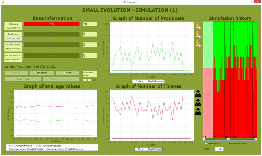
Population Level 20
The Producers become extinct after 34 cycles. The number of Producers range from 2 to 12, and Thieves 8 to 18.
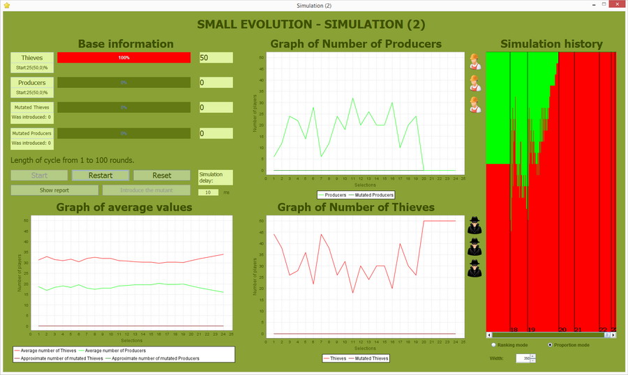
Population Level 50
The Producers become extinct after 20 cycles. The number of Producers range from 6 to 30, and Thieves 20 to 44.
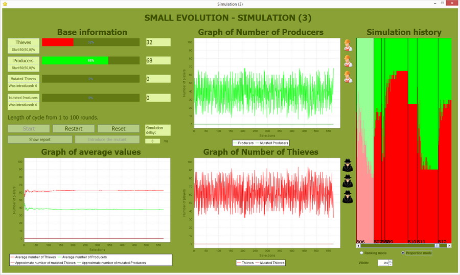
Population Level 100
There were no extinction of Producers, even after 600 cycles. The number of Producers range from 5 to 70, and Thieves 30 to 95.
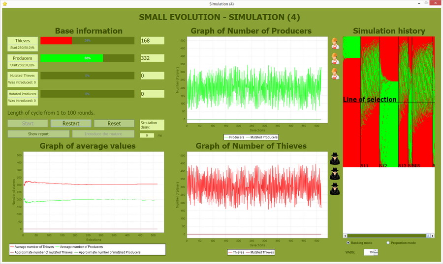
Population Level 500
There were no extinction of Producers after 600 cycles. The number of Producers range from 50 to 350, and Thieves 150 to 450.
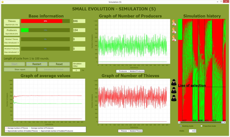
Population Level 1000
There were no extinction of Producers after 425 cycles. The number of Producers range from 110 to 700, and Thieves 300 to 890.
Based on the above simulations one can discover the following pattern:
of the extinction of the Producers.
Analysis without mutation - varying Selection Function Strength:

Taking into account the results of the two previous simulations, for the third one we will assume that the cycle length will be in the range of 1 - 100 and the population level will be relatively large = 1000. Now let's see how the population is affected by a change in the selection function strength.
At this point, it is worth paing attention to the restoration algorithm of the population. Because if the selection function strength is:
-
Weak - the population loses, for example, only 20% of its members. In this case, the process of the restoration of the population will have to restore only the missing 20% from the remaining 80% - so only some of them will be cloned.
-
Strong - the population loses, for example, 85% of its members. In this case, the process of the restoration of the population will have to restore the missing 85% from the remaining 15% - so many of them will be cloned numerous times.
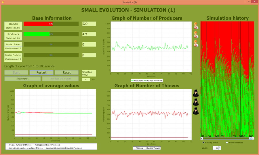
Selection Function Strength 80%
Because the leading 80% of participants are selected, it can be termed "very weak". The ratio of Producers to Thieves hovers around the average, and it is unlikely that Thieves will dominate the population.
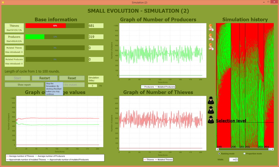
Selection Function Strength 60%
Because the leading 60% of participants are selected, it can be termed "weak". The ratio of Producers to Thieves hovers around the average, and it is unlikely that Thieves will dominate the population. However, in comparison to the previous simulation, amplitude growth is noticeable.

Selection Function Strength 40%
With the standard setting of 50% Selection Function Strength it did not cause the Thieves to dominate. This time, with a "strong" Selection Function Strength of 40% of the leading participants, the dominance of the Thieves is noticeable after 28 cycle.
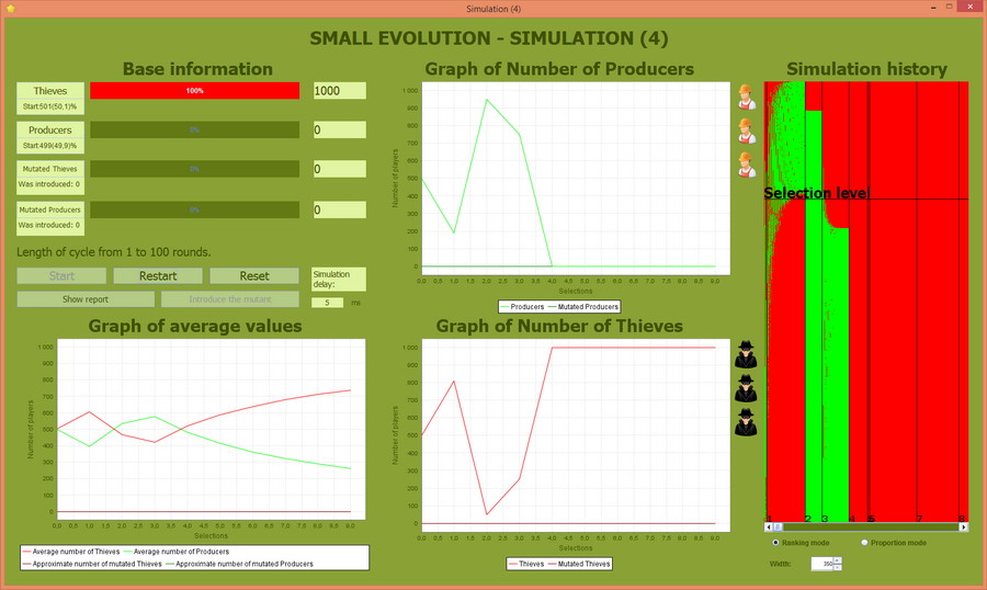
Selection Function Strength 20%
Because the leading 20% of participants are selected, it can be termed "very strong". The process of the restoration of the population clones only the best 20%. As you can see, the domination by the Thieves is almost immediate.
Based on the above simulations one can discover the following pattern:
the probability of the extinction of the Producers.
Analysis with mutation - Introduction of a Negative Mutant:

The Negative Mutant is one that gets less points at each Single meeting game. After introducing the Mutant, we have three types of individuals in the population: Producers, Thieves and one newly introduced Negative Mutant.
Both Thieves and Producers can be mutated. The mutation itself can be:
-
Half-Negative - a Mutant will get less points only when meeting Thieves, the number of points earned during the meetings with Producers will not change; Note that there are 4 types of such mutants.
-
Full-Negative - a Mutant will get less points when meeting Thieves and Producers. Note that there are 2 types of such mutants.
Because the Thieves are more populous, we mutated one of them.
For simulation, the parameters will be set to ensure the relative stability of the composition of the population. That is, they will not cause the Thieves to overwhelm the population too quickly. Let's set them as follows:
Cycle Length - from 1 to 100 rounds
Population level - 500 participants
Selection function strength - 50% [50% of the leading participants are selected]
The mutation is Full-Negative which means that the mutated Thief gets one point less than normal in both types of meetings.
The initial settings window looks as follows:
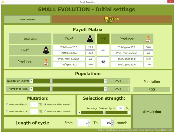
Negative Mutation - settings window
During the simulation the Full-Negative Mutant Thief was introduced twice. The number of mutants in the population is shown at the bottom of the window "Graph of Number of Thieves".
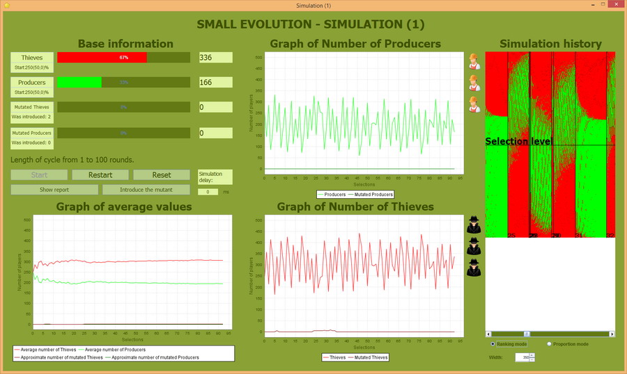
Negative Mutation - simulation screen
On the screen above you can see that the Full-Negative Mutant Thief survives in the first case for one cycle and in the other for 9, and even manages to increase his number in the population to 4 individuals. But in both cases mutants are dying out anyway.
The programme allows you to take a look at how Full-Negative Mutant Thieves are ranked. This is illustrated by the "Simulation history" window where mutants are represented by darker pixels.
Based on the above simulations one can discover the following pattern:
does not change the composition of the population.
Negative Mutants eventually become extinct.
Analysis with mutation - Introduction of a Half-Positive Mutant:

This time let's introduce the Half-Positive Mutant Producer. "Half" because this Mutant gets one more point but only in meetings with other Producers.
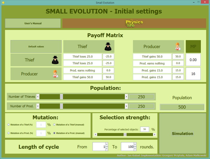
Half-Positive Mutant Producer - settings window
Numeric values that tell how and where the Mutant gets more points are shown on the right side of the Payoff Matrix.
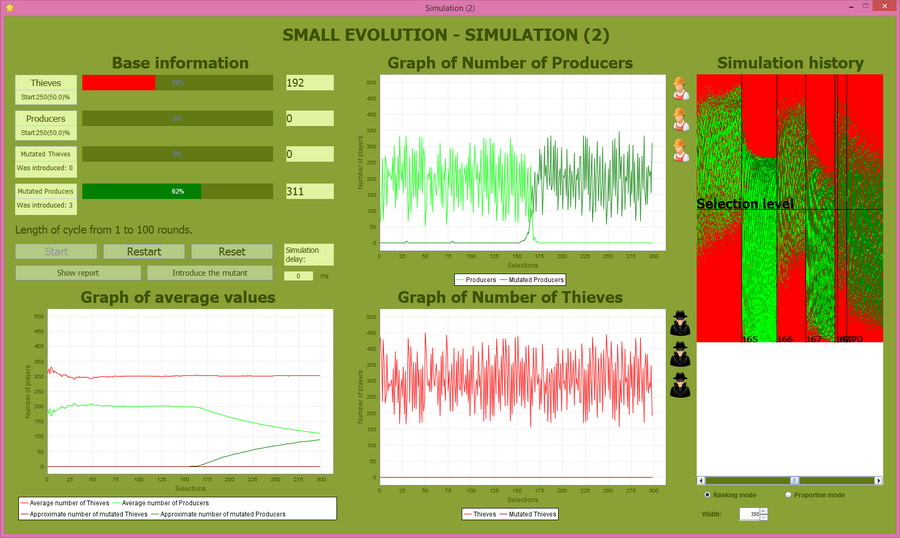
Half-Positive Mutant Producer - simulation window
It can be seen that three attempts were made to introduce the Half-Positive Mutant Producer to the population. In the first two cases the Mutants died out, but the third mutant's offspring completely dominated the Producer population. This domination took place in 25 rounds, that is to say that a population of 500 participants was dominated by Mutants in only 25 generations. This is not an exponential growth, for if it was, then the domination would take place in the 10th generation.
Based on the above simulations one can discover the following pattern:
to survive the selection function strength,
his descendants will dominate the population.
The definiendum of this mechanism is evolutionary ratchet.
Analysis with mutation - Introduction of a Full-Positive Mutant:

We will perform this simulation by introducing the Full-Positive Mutant Producer. This mutant gains one more point in both type of meetings.
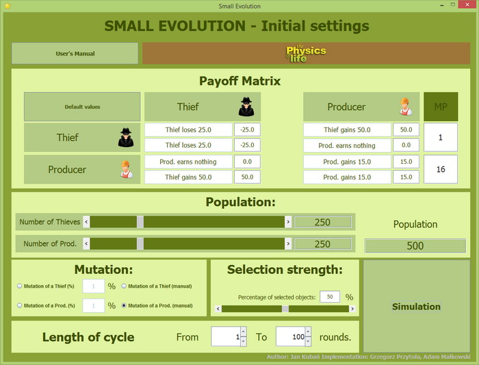
Full-Positive Mutant Producer - settings window
The numerical values that tell you how and where the mutant is better are shown on the right side of the Payoff Matrix.
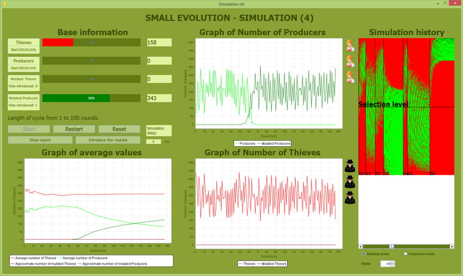
Full-Positive Mutant Producer - simulation window
In this case, the Mutants dominate the whole population after 14 generations, twice as quickly as the Half-Positive Mutants in the previous simulation. The curious fact is that the Full-Positive Mutant is not always fortunate enough to be selected. In doing so many simulations with these settings, it turned out that sometimes a mutant fails to break through the selection. This is because when the Full-Positive Mutant Producer is introduced to the population, it may meet relatively few Thieves. Thieves are much more likely to meet with Producers and therefore quickly rise to the top of the ranking list. If the Full-Positive Mutant Producer is more likely to meet Thieves than Producers, then his points tally will grow slower than the Producers, who mainly meet other Producers. This may not allow the Full-Positive Mutant Producer to gain a high enough rank in the list that would enable him to be selected.
Based on the above simulations one can discover the following pattern:
will dominate the population almost exponentially.
Sometimes, a Fully-Positive Mutant may not be fortunate enough
to survive the selection function strength.
Small Evolution - "Realistic" Payoff Matrix

Basic assumptions:
As in the classic example of this game, proposed by John Maynard Smith, there are only two types of strategy Producers and Thieves, however, there is a different Payoff Matrix, which looks more realistic:
| "Small Evolution" – "Realistic" Payoff Matrix | ||
| Thief | Thief loses 1 (-1) Thief loses 1 (-1) |
Thief gains 50 (+50) Producer loses 50 (-50) |
| Producer | Producer loses 50 (-50) Thief gains 50 (+50) |
Producer gains 10 (+10) Producer gains 10 (+10) |
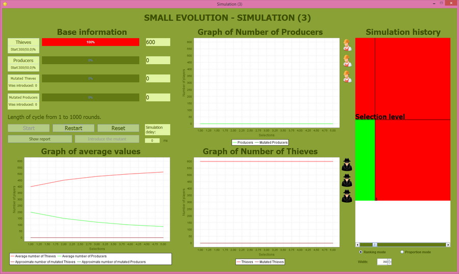
Simulation with "Realistic" Payoff Matrix - cycle from 1 to 1000 rounds
With such a Payoff Matrix it is evident that Producers will become extinct quickly. Does it somehow undermine our previous considerations? Absolutely not. This only shows how much depends upon the Payoff Matrix and leads to the next most important conclusion.
If the producers are extinct, then it is obvious that the population will only consist of Thieves. As a result, all single-meeting games will be played between Thieves. So none of the Thieves will ever accumulate a positive number of points, which are needed to survive even in real life. That is, no one will be able to survive. If the Thieves make the Producers extinct, they will also eventually die out, unless ... they will start playing different games in a different way, with different rules. This is a vital conclusion that the Thieves will find themselves in coercion of cooperation.
Small Evolution - Conclusions

Here are the main conclusions from the simulations:
-
Increasing the number of rounds in the cycle increases the probability of the extinction of the Producers.
-
Increasing the population level reduces the probability of the extinction of the Producers.
-
Increasing the selection function strength increases the probability of the extinction of the Producers.
-
The introduction of the Negative Mutant, in the long term, does not change the composition of the population. Negative Mutants eventually become extinct.
-
If the Half-Positive Mutant is fortunate enough to survive the selection function strength, his descendants will dominate the population.
-
The descendants of a Fully-Positive Mutant of a Producer will dominate the population almost exponentially. Sometimes, such a Mutant may not be fortunate enough to survive the selection function strength.
Please note that these conclusions are derived from the simulations limited by:
- the given values of the parameters,
- the given assumptions,
- and the given algorithms.
The factor of furtility rates was not touched upon, however, I feel it may have given interesting results.
Another very important conclusion is that reductionist thinking is absolutely insufficient to understand the population phenomena. To understand them, one has to extend their conceptual apparatus with, at least, multitudinal thinking and game thinking.
History of Human Populations

Here is an interesting chart showing the history of the world's dominating human populations. It highlights how dominant populations increased, decreased, emerged and occasionally became exitinct. It is available on: The Entire History of the World — Distilled Into a Single Gorgeous Chart. In its nature it is like the charts of our computer simulation.

Links

-
Human and nature dynamics (HANDY): Modeling inequality and use of resources in the collapse or sustainability of societies
There are widespread concerns that current trends in resource-use are unsustainable, but possibilities of overshoot/collapse remain controversial. Collapses have occurred frequently in history, often followed by centuries of economic, intellectual, and population decline. Many different natural and social phenomena have been invoked to explain specific collapses, but a general explanation remains elusive.
In this paper, we build a human population dynamics model by adding accumulated wealth and economic inequality to a predator–prey model of humans and nature. The model structure, and simulated scenarios that offer significant implications, are explained. Four equations describe the evolution of Elites, Commoners, Nature, and Wealth. The model shows Economic Stratification or Ecological Strain can independently lead to collapse, in agreement with the historical record.
The measure “Carrying Capacity” is developed and its estimation is shown to be a practical means for early detection of a collapse. Mechanisms leading to two types of collapses are discussed. The new dynamics of this model can also reproduce the irreversible collapses found in history. Collapse can be avoided, and population can reach a steady state at maximum carrying capacity if the rate of depletion of nature is reduced to a sustainable level and if resources are distributed equitably.
